Outputting simulated accumulated precipitation at upper levels in WRF
This tutorial describes how to modify the WRF model source code to output a new 3D
variable, RAINNC3d, that stores accumulated total grid-scale precipitation
at every model level in addition to the standard surface output. Throughout the tutorial
I will share line numbers from the WRF that I used for modifications, but it is likely that
line numbers in different WRF installations or versions will be different.
This tutorial is for the Thompson microphysics scheme and requires changes to four files:
Registry/Registry.EM_COMMONphys/module_mp_thompson.Fphys/module_microphysics_driver.Fdyn_em/solve_em.F
Using similar techniques, this modification can be made for other microphysics schemes as well.
1 Modify the Registry
The WRF Registry (Registry/Registry.EM_COMMON) defines all model variables.
The surface accumulated precipitation is called RAINNC; add a new 3D
variable called RAINNC3d to store precipitation at all levels.
Add the following line to the registry:
#=========================================================
# Modified by Michael Wasserstein 2 Mar 2026 — precip at a upper levels
state    real  RAINNC3d   ikj   misc   1   -   rh01du   "RAINNC3d"   \
         "ACCUMULATED TOTAL GRID SCALE PRECIPITATION at levels"   "mm"
#=========================================================
The ikj dimension specifier makes this a 3D variable covering all
horizontal grid points and all vertical levels in the domain, in contrast to the standard
RAINNC variable for surface precipitation, which only has i and k.
2 Modify the Thompson Microphysics Scheme
The next step is to open the Thompson microphysics code,
phys/module_mp_thompson.F, and find every occurrence of
RAINNC and add the 3D counterpart alongside it.
- Add
RAINNC3dto the driver subroutine (line 979)
SUBROUTINE mp_gt_driver(qv, qc, qr, qi, qs, qg, ni, nr, nc,       &
                        nwfa, nifa, nwfa2d, nifa2d,               &
                        th, pii, p, w, dz, dt_in, itimestep,      &
                        RAINNC, RAINNCV,                           &
                        RAINNC3d,  &  ! Michael Wasserstein Feb 24 2026
                        SNOWNC, SNOWNCV,                           &
GRAUPELNC, GRAUPELNCV, SR, &- Declare
RAINNC3das a 3D intent variable (line 1022)
REAL, DIMENSION(ims:ime, jms:jme), INTENT(INOUT):: &
                    RAINNC, RAINNCV, SR
!..==================================================================
!.. Michael Wasserstein modified feb 24 2026 for precip at upper levels
REAL, DIMENSION(ims:ime, kms:kme, jms:jme), INTENT(INOUT):: &
                    RAINNC3d
!..==================================================================-
In the Thompson scheme, precipitation is calclated for each precipitating hydrometeor type,
including rain, snow, graupel, and ice. Here, we create 3D variables analogous to the
1D variables for each hydrometeor type. The
pcp*variables will store an entire 3D array, and theppt*variables will be used for the summation of preciptiation (line 1078).
REAL, DIMENSION(its:ite, jts:jte):: pcp_ra, pcp_sn, pcp_gr, pcp_ic
!=================================================================
!.. Modified by Michael Wasserstein to get precip at upper levels
!.. February 24, 2026
REAL, DIMENSION(its:ite, kts:kte, jts:jte) :: pcp_ra3d, pcp_sn3d, &
                                              pcp_gr3d, pcp_ic3d
REAL, DIMENSION(kts:kte) :: pptrain3d, pptsnow3d, pptgraul3d, pptice3d
!=================================================================- Initialize precipitation accumulators to zero (line 1163).
!================================================================
!.. Michael Wasserstein Feb 24 2026 edits
pptrain3d  = 0.
pptsnow3d  = 0.
pptgraul3d = 0.
pptice3d   = 0.
!================================================================- Pass the 3D arrays into
mp_thompsonfunction (line 1232).
call mp_thompson(qv1d, qc1d, qi1d, qr1d, qs1d, qg1d, ni1d,    &
             nr1d, nc1d, nwfa1d, nifa1d, t1d, p1d, w1d, dz1d, &
             pptrain, pptsnow, pptgraul, pptice,               &
             pptrain3d, pptsnow3d, pptgraul3d, pptice3d,    & ! Wasserstein
#if ( WRF_CHEM == 1 )
             rainprod1d, evapprod1d,                           &
#endif- Here, the modifications store the 3D results in the same way as the 2D results. (line 1244)
pcp_ra(i,j) = pptrain
pcp_sn(i,j) = pptsnow
pcp_gr(i,j) = pptgraul
pcp_ic(i,j) = pptice
!===========================================================
!.. Michael Wasserstein modified 24 feb 2026
do k = kts, kte
  pcp_ra3d(i,k,j) = pptrain3d(k)
  pcp_sn3d(i,k,j) = pptsnow3d(k)
  pcp_gr3d(i,k,j) = pptgraul3d(k)
  pcp_ic3d(i,k,j) = pptice3d(k)
enddo
!===========================================================
RAINNCV(i,j) = pptrain + pptsnow + pptgraul + pptice
RAINNC(i,j)  = RAINNC(i,j) + pptrain + pptsnow + pptgraul + pptice
!===========================================================
!.. Michael Wasserstein modified 24 feb 2026
do k = kts, kte
  RAINNC3d(i,k,j) = RAINNC3d(i,k,j) + pptrain3d(k) + pptsnow3d(k) + &
                                       pptgraul3d(k) + pptice3d(k)
enddo
!===========================================================- Update the
mp_thompsonsubroutine (line 1491).
subroutine mp_thompson (        &
                    qv1d, qc1d, qi1d, qr1d, qs1d, qg1d,         &
                    ni1d, nr1d, nc1d, nwfa1d, nifa1d,            &
                    t1d, p1d, w1d, dzq,                          &
                    pptrain, pptsnow, pptgraul, pptice,           &
pptrain3d, pptsnow3d, pptgraul3d, pptice3d, & ! Wasserstein- Declare the added 3D variables in the subroutine (line 1515).
REAL, INTENT(INOUT):: pptrain, pptsnow, pptgraul, pptice
! Michael Wasserstein Feb 26 2026
REAL, DIMENSION(kts:kte), INTENT(INOUT):: &
      pptrain3d, pptsnow3d, pptgraul3d, pptice3d
The microphysics scheme accumulates precipitation for each hydrometeor type (rain,
ice, snow, graupel) based on whether the mixing ratio exceeds a threshold
R1 and using the sedimentation rate at each level. After each
existing 2D accumulation line, we add the following edits for 3D accumulation:
Rain (line 3522)
if (rr(kts).gt.R1*1000.) &
  pptrain = pptrain + sed_r(kts)*DT*onstep(1)
!.. Michael Wasserstein edits Feb 24 2026
do k = kte, kts, -1
  if (rr(k).gt.R1*1000.) &
    pptrain3d(k) = pptrain3d(k) + sed_r(k)*DT*onstep(1)
enddo
Ice (line 3580)
if (ri(kts).gt.R1*1000.) &
  pptice = pptice + sed_i(kts)*DT*onstep(2)
!.. Michael Wasserstein edits Feb 24 2026
do k = kte, kts, -1
  if (ri(k).gt.R1*1000.) &
    pptice3d(k) = pptice3d(k) + sed_i(k)*DT*onstep(2)
enddo
Snow (line 3615)
if (rs(kts).gt.R1*1000.) &
  pptsnow = pptsnow + sed_s(kts)*DT*onstep(3)
!.. Michael Wasserstein edits Feb 24 2026
do k = kte, kts, -1
  if (rs(k).gt.R1*1000.) &
    pptsnow3d(k) = pptsnow3d(k) + sed_s(k)*DT*onstep(3)
enddo
Graupel (line 3649)
if (rg(kts).gt.R1*1000.) &
  pptgraul = pptgraul + sed_g(kts)*DT*onstep(4)
!.. Michael Wasserstein edits Feb 24 2026
do k = kte, kts, -1
  if (rg(k).gt.R1*1000.) &
    pptgraul3d(k) = pptgraul3d(k) + sed_g(k)*DT*onstep(4)
enddo
3 Modify module_microphysics_driver.F
Next, we open phys/module_microphysics_driver.F and search for every occurrence
of rainnc, adding RAINNC3d alongside each one.
- Add to the microphysics_driver subroutine (
SUBROUTINE microphysics_driver;line 95)
                  ,rainnc,    rainncv                                &
,RAINNC3d & ! Michael Wasserstein 2/24/26- Declare the variable in the subroutine (line 676)
REAL, DIMENSION( ims:ime , kms:kme, jms:jme ) :: RAINNC3d ! Michael Wasserstein Mar 2 2026- Pass
RAINNC3din the microphysics driver call (line 1055)
                 RAINNC=RAINNC,                      &
                 RAINNCV=RAINNCV,                    &
                 RAINNC3d=RAINNC3d,                  & ! Michael Wasserstein 3d rain
And again at line 1134
RAINNC3d=RAINNC3d, & ! Michael Wasserstein 3d rain4 Modify solve_em.F
The last file to modify is dyn_em/solve_em.F. The microphysics driver is called near
line 3603. Only one small addition is needed at line 3692 to pass the
new variable in the microphysics driver:
     &        , RAINNC=grid%rainnc, RAINNCV=grid%rainncv                 &
     &        , RAINNC3d=grid%rainnc3d                                   & ! Michael Wasserstein Feb 24 2026
5 Reconfigure and Recompile
After making all modifications, reconfigure and recompile WRF. Once the model
is rerun, the output will contain a new variable RAINNC3D giving the
simulated effective accumulated precipitation at every vertical level in the domain.
Applications: Sub-Cloud Sublimation
One Useful application for this includes understanding the influence of sub-cloud sublimation of hydrometeors. For instance, one simulation of a March 2019 winter storm in the Wasatch shows precipitation loss over the Salt Lake Valley due to sublimation:
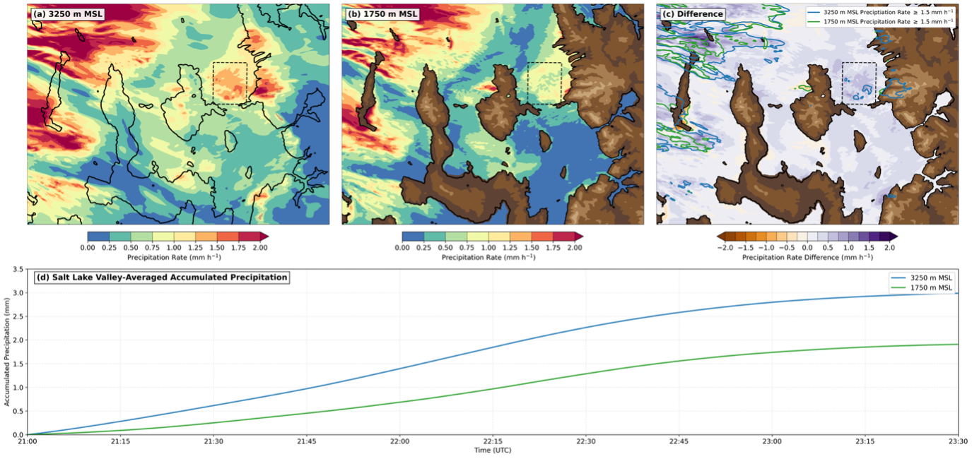
In Fig. 1a, notice how effective precipitation rates at 3250 m MSL (~2000 m AGL) for the analysis time are generally between 0.75 and 1.75 mm h−1 over the black dashed box outlining the Salt Lake Valley. But at 1750 m MSL (~500 m AGL), precipitation rates are lower due to sub-cloud sublimation (Fig. 1b). That can be seen by looking at a difference plot of the rates at 3250 m MSL – the rates at 1750 m MSL (Fig. 1c) or a time series plot indicating the effective accumulated precipitation over time (Fig. 1d), which indicates greater accumulated precipitation at 3250 m MSL (blue line) compared to 1750 m MSL (green line).
This microphysical process can also viewed in a cross section over the Salt Lake Valley:
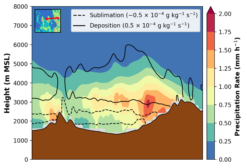
The cross-section in Fig. 2 shows the highest effective precipitation rates near 3000 m MSL, decreasing with height loss toward the surface. Sublimation (dashed black contour) is greatest between roughly 1800 and 2500 m MSL over the Salt Lake Valley, consistent with the dashed contour in Fig. 2, indicating sublimation rates ≤ −0.5 × 10⁻⁴ g kg−1 s−1.